A simple Bayesian inference example with Grid approximate, from scratch
why Bayesian?
Using probability methods to solve statistical problems.
For many problems in real life, we normally have an educated guess (prior), and this prior is helpful to our final guess/prediction. Through observing new data/evidence, we are upating our guess(prior), and the updated guess is posterior.
In the Bayesian inference workflow, we treat problems interatively, that is, we can get a new posterior through new observations, and then use it as the (new) prior.
Bayes' rule
Bayes' theorem begins with conditional probability.
because:
\[ Pr(A|B) = \frac{Pr(A\cap B)}{Pr(B)} \] \[ Pr(B|A) = \frac{Pr(B\cap A)}{Pr(A)} \]
then: \[ Pr(A|B)Pr(B) = Pr(A\cap B) \] \[ Pr(B|A)Pr(A) = Pr(B\cap A) \]
so: \[ Pr(A|B)Pr(B) = Pr(B|A)Pr(A) \]
Bayes' rule: \[ Pr(A|B) = \frac{Pr(B|A)Pr(A)}{Pr(B)} \]
Bayesian inference
The core of Bayesian Statistics is to update our understanding of unknown parameters through new observational data/evidence.
For example, we are curious to know a unknow (\theta), and we guess its prior is \(Pr(\theta)\). We have a sequence of observations (D). We hope \(D\) can help us better to understand \(Pr(\theta)\). It is that we are intersted in \(Pr(\theta|D)\). According to Bayes' rule, we know:
\[ Pr(\theta|D) = \frac{Pr(D|\theta)Pr(\theta)}{Pr(D)} \]
where:
- \(Pr(\theta)\): prior of \(\theta\), that is our guess of \(\theta\) without any observations \(D\).
- \(Pr(\theta|D)\): posterior of \(\theta\), that is our updated guess of \(\theta\) via any observations \(D\).
- \(Pr(D|\theta)\): likelihood, that is the probability of \(D\) under a certain \(\theta\).
- \(Pr(D)\): observations/evidence, that is the probability of \(D\) under all possible \(\theta\).
example
Statistical Rethinking by Richard McElreath
The example is from Statistical Rethinking by Richard McElreath. Here, I derive it from scratch and only using math.
1. QUESTION AND GOAL
There is a globe, and we want to know how much of the surface is covered in water.
You will toss the globe up in the air. When you catch it, you will record whether or not the surface under your right index finger is water \(W\) or land \(L\). Then you toss the globe up in the air again and repeat the procedure.
observations are: [ W \quad L\quad W\quad W\quad W\quad L\quad W\quad L\quad W ]
2. DATA INFORMATION
- The true proportion of water covering the globe is \(p\). (as \(\theta\) in the above work)
- A single toss of the globe has a probability \(p\) of producing a water (\(W\)) observation. It has a probability \(1-p\) of producing a land (\(L\)) observation. (There are only two events: \(W\) or \(L\))
- Each toss of the globe is independent of the others.
- The total number of observations is \(N=W+L\). In this case, \(N=9, W=6, L=3\).
3. MODELING
the assumption of the likelihood \(Pr(W,L|p)\):
\[ W \thicksim Binomail(N,p) \]
the binomial distribution is rather special for counting binary events.
About \(binomial\) distribution: \[ Pr(k,n,p)=Pr(X=k)=\frac{n!}{k!(n-k)!}p^k(1-p)^{(n-k)} \] The probability of getting exactly \(k\) successes in \(n\) independent \(Bernoulli\) trials (with the same rate \(p\)). In our case, the probability of seeing \(k=W\) in \(n=N=W+L\) observations is: \[ Pr(W,L,p)=Pr(X=W)=\frac{(W+L)!}{W!L!}p^W(1-p)^{L} \]
the prior of \(p\):
\[ Pr(p) \thicksim Uniform(0,1) \]
a flat distribution.
the posterior of \(p\) through observations \(W\) and \(L\):
\[ Pr(p|W,L) =\frac{Pr(W,L|p)Pr(p)}{Pr(W,L)} \]
4.GRID APPROXIMATE
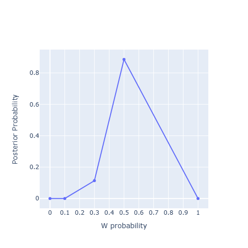
the grid of \(p\) is \([0, 0.1, 0.3, 0.5, 1]\)
corresponding prior \(Pr(p)\) is \([1, 1, 1, 1, 1]\)
corresponding likelihood:
-
\(p_1=0\) \[ Pr(W,L|p_1)=\frac{(W+L)!}{W!L!}p_1^W(1-p_1)^{L}=0 \]
-
\(p_2=0.1\) \[ Pr(W,L|p_2)=\frac{(W+L)!}{W!L!}p_2^W(1-p_2)^{L}=\frac{9!}{6!3!}0.1^6\times 0.9^{3}=0.00006123600000000004 \]
-
\(p_3=0.3\) \[ Pr(W,L|p_3)=\frac{(W+L)!}{W!L!}p_3^W(1-p_3)^{L}=\frac{9!}{6!3!}0.1^6\times 0.9^{3}=0.02100394799999999 \]
-
\(p_4=0.5\) \[ Pr(W,L|p_4)=\frac{(W+L)!}{W!L!}p_4^W(1-p_4)^{L}=\frac{9!}{6!3!}0.1^6\times 0.9^{3}=0.1640625 \]
-
\(p_5=1\) \[ Pr(W,L|p_5)=\frac{(W+L)!}{W!L!}p_5^W(1-p_5)^{L}=\frac{9!}{6!3!}0.1^6\times 0.9^{3}=0 \]
\(Pr(W,L)\) (as \(Pr(D)\) in the above work):
\[
\begin{align*}
Pr(W,L) &= \displaystyle\sum_{i=1}^{5} Pr(W,L|p_i)\times Pr(p_i) \
&= 0\times 1 +0.00006123600000000004\times 1 + 0.02100394799999999\times 1 + 0.1640625\times 1 + 0\times 1\
&= 0.185127684
\end{align*}
\]
Pr(p|W,L)
-
\(p_1=0\) \[ Pr(p_1|W,L)=\frac{Pr(W,L|p_1)Pr(p_1)}{Pr(W,L)}=\frac{0\times 1}{ 0.185127684}=0 \]
-
\(p_2=0.1\) \[ Pr(p_2|W,L)=\frac{Pr(W,L|p_2)Pr(p_2)}{Pr(W,L)}=\frac{0.00006123600000000004\times 1}{ 0.185127684}=0.00033077710840913473 \]
-
\(p_3=0.3\) \[ Pr(p_3|W,L)=\frac{Pr(W,L|p_3)Pr(p_3)}{Pr(W,L)}=\frac{0.02100394799999999\times 1}{ 0.185127684}=0.11345654818433311 \]
-
\(p_4=0.5\) \[ Pr(p_4|W,L)=\frac{Pr(W,L|p_4)Pr(p_4)}{Pr(W,L)}=\frac{0.1640625\times 1}{ 0.185127684}=0.8862126747072577 \]
-
\(p_5=1\) \[ Pr(p_5|W,L)=\frac{Pr(W,L|p_5)Pr(p_5)}{Pr(W,L)}=\frac{0\times 1}{ 0.185127684}=0 \]
visualization